Housing Subsidy

Introduction

The Department of Housing and Community Development (HCD) in Emil City is launching a home repair tax credit program, and they want to reach out to those who are most likely to take this credit at a low cost. When reaching out randomly, only 11% of the homeowners take this credit and the unsuccessful reach out also wastes a large amount of money.

In order to make the most use of the housing subsidy and create a satisfying benefit, I will build a logistic regression model to predict under given features whether a homeowner will take the credit or not.

Code

knitr::opts_chunk$set(echo = TRUE)
options(scipen=10000000)
library(tidyverse)
library(kableExtra)
library(caret)
library(knitr) 
library(pscl)
library(plotROC)
library(pROC)
library(lubridate)
library(ggcorrplot) 
library(vcd)
library(grid)

Code

palette5 <- c("#264653","#2a9d8f","#e9c46a",'#f4a261',"#e76f51")
palette4 <- c("#264653","#2a9d8f","#e9c46a","#e76f51")
palette2 <- c("#264653","#2a9d8f")

churn <- read.csv('/Users/mr.smile/Desktop/UPENN/FALL23/MUSA508/musa_5080_2023-main/Housing Subsidy/churnBounce.csv')

house_sub <- read.csv('/Users/mr.smile/Desktop/UPENN/FALL23/MUSA508/musa_5080_2023-main/Housing Subsidy/housingSubsidy.csv')

Data Visualization

Firstly, we want to figure out if there’s significantly feature difference in the groups whether they entered the program, which is useful and effective to determine the potential correlation between different variables and choices. The bar plot showing the median value of the feature, which represent the average situation, doesn’t tell much difference in whether enter the program. Besides, we can find that the group entering the program has a slightly higher median age and lower spend on repairs than the group not entering the program.

Code

house_sub %>%
  dplyr::select(y,age, spent_on_repairs, cons.price.idx, cons.conf.idx) %>%
  gather(Variable, value, -y) %>%
    ggplot(aes(y, value, fill=y)) + 
      geom_bar(position = "dodge", stat = "summary", fun = "median") + 
      facet_wrap(~Variable, scales = "free") +
      scale_fill_manual(values = palette2) +
      labs(x="Churn", y="Value", 
           title = "Feature associations with the likelihood of entering the program",
           subtitle = "(continous outcomes)") +
      theme(legend.position = "none")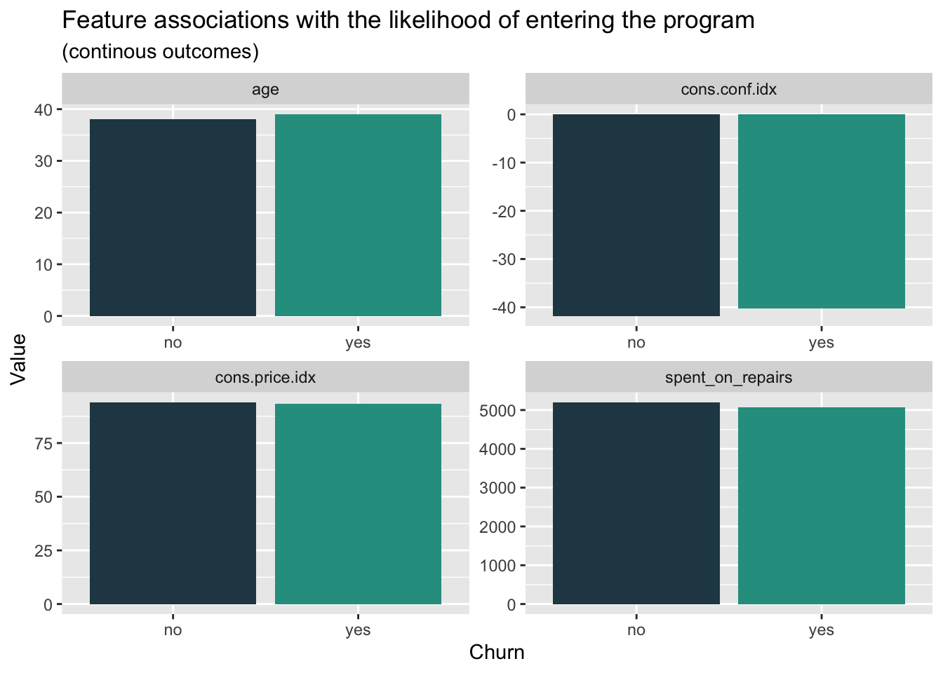

When it comes to the density plot of the features above, we can find two groups have apparent differences in the distribution. The group entering the program has a relatively lower distribution in the age from 30 to 50 years. As for the spend on repairs, we can clearly find that the group entering the program has an obviously lower distribution in the higher spend interval. When we focus on the economic background of the decision, we can find that the lower confidence index, which represent the relatively low consumption desire, have less influence on the group entering the program. Meanwhile, the higher consumer price index has more association with the rejection to enter the program.

Code

house_sub %>%
    dplyr::select(y,age, spent_on_repairs, cons.price.idx, cons.conf.idx) %>%
    gather(Variable, value, -y) %>%
    ggplot() + 
    geom_density(aes(value, color=y), fill = "transparent") + 
    facet_wrap(~Variable, scales = "free") +
    scale_fill_manual(values = palette2) +
    labs(title = "Feature distributions enter vs. no enter",
         subtitle = "(continous outcomes)")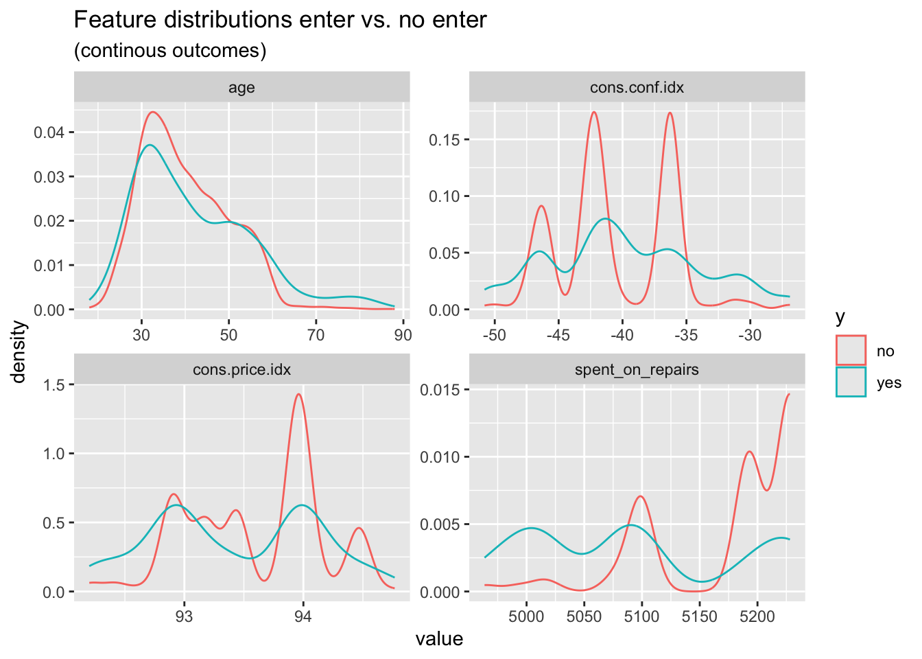

When we look at the count plot for different features related to whether entering the program, we can find that, in general, the group not entering the program has more members than that entering the program. In the job feature, we can find that the gap in some field is more extreme like administor, blue-collar, and technican.

Code

house_sub %>%
    dplyr::select(y, marital,job,taxLien,poutcome) %>%
    gather(Variable, value, -y) %>%
    count(Variable, value, y) %>%
      ggplot(., aes(value, n, fill = y)) +   
        geom_bar(position = "dodge", stat="identity") +
        facet_wrap(~Variable, scales="free") +
        scale_fill_manual(values = palette2) +
        labs(x="Click", y="Value",
             title = "Feature associations with the likelihood of entering",
             subtitle = "Categorical features") +
        theme(axis.text.x = element_text(angle = 45, hjust = 1))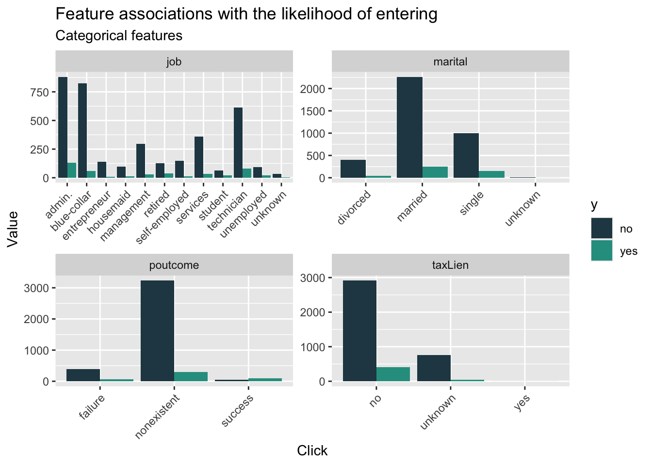

Data Modeling

Feature Engineering

From the initial data visualization, we could hardly figure out the significantly difference between two different groups. Therefore, it’s essential to engineering the feature to improve further model performance. As for the education, jobs and pdays, which both have many categories, I re-categorize these feature into fewer categories. What’s more, I standardize the cpi and cci indicator to improve the interpretablity.

Code

house_sub$cons.price.idx_s <- scale(house_sub$cons.price.idx)
house_sub$cons.conf.idx_s <- scale(house_sub$cons.conf.idx)
house_sub$poutcome_new <- ifelse(house_sub$poutcome == "success", 1, 0)
house_sub <- 
  house_sub %>% 
  mutate(education,
         education_new = case_when(education == "basic.4y" ~ "medium",
                               education == "basic.6y" ~ "medium",
                               education == "basic.9y" ~ "high",
                               education == "high.school" ~ "high", 
                               education == "professional.course" ~ "high",
                               education == "university.degree" ~ "very high",
                               education == "illiterate"  ~ "low", 
                               education == "unknown" ~ "low"))%>%
  mutate(job,
         job_new = case_when(job == "retired" ~ "low income",
                         job == "unemployed" ~ "low income", 
                         job =="unknown" ~ "low income", 
                         job == "student" ~ "low income",
                         job == "housemaid" ~ "medium income",
                         job == "blue-collar" ~ "medium income",
                         job == "services" ~ "medium income",
                         job == "technician" ~ "high income",
                         job ==  "management" ~ "high income",
                         job == "admin." ~ "high income",
                         job == "entrepreneur" ~ "very high income", 
                         job == "self-employed" ~ "medium income")) %>%
  mutate(pdays,
         pdays_new = case_when(pdays == "0"  ~ "0-6",
                           pdays == "1" ~ "0-6", 
                           pdays == "2" ~ "0-6", 
                           pdays == "3" ~ "0-6", 
                           pdays == "4" ~ "0-6", 
                           pdays == "5" ~ "0-6", 
                           pdays == "6" ~ "0-6", 
                           pdays == "7" ~ "7-15",
                           pdays == "9"  ~ "7-15",
                           pdays == "10"  ~ "7-15", 
                           pdays == "11"  ~ "7-15", 
                           pdays == "12"  ~ "7-15", 
                           pdays == "13"  ~ "7-15", 
                           pdays == "14"  ~ "7-15", 
                           pdays == "15"  ~ "7-15", 
                           pdays == "17" ~ "16-21", 
                           pdays == "18" ~ "16-21",
                           pdays == "19" ~ "16-21", 
                           pdays == "21"~ "16-21", 
                           pdays == "16" ~ "16-21",
                           pdays == "999" ~ "unknown"))

Training and Test split

After feature engineering, I split the dataset into training and test one with 65/35 for further data modeling. To compare the performance of new feature, I test the performance of both model using the raw features in the dataset and model with variables after feature engineering and selection.

Code

trainIndex <- createDataPartition(house_sub$y, p = .65,
                                  list = FALSE,
                                  times = 1)
houseTrain <- house_sub[ trainIndex,]
houseTest  <- house_sub[-trainIndex,]

Code

set.seed(3426)
tempModel <- glm(y_numeric ~ .,
                  data=houseTrain %>% 
                    dplyr::select(-X,- y,-cons.price.idx_s,-cons.conf.idx_s,
                                  -poutcome_new,-education_new,-job_new,-pdays_new),
                  family="binomial" (link="logit"))

testProbs_raw <- data.frame(Outcome = as.factor(houseTest$y_numeric),
                        Probs = predict(tempModel, houseTest, type= "response"))
summary(tempModel)

Call:
glm(formula = y_numeric ~ ., family = binomial(link = "logit"), 
    data = houseTrain %>% dplyr::select(-X, -y, -cons.price.idx_s, 
        -cons.conf.idx_s, -poutcome_new, -education_new, -job_new, 
        -pdays_new))

Coefficients:
                                 Estimate   Std. Error z value Pr(>|z|)    
(Intercept)                  -193.7565741  127.7984723  -1.516 0.129491    
age                             0.0142384    0.0086150   1.653 0.098383 .  
jobblue-collar                 -0.3467856    0.2861796  -1.212 0.225598    
jobentrepreneur                -0.5024294    0.4766389  -1.054 0.291833    
jobhousemaid                    0.0665795    0.4920445   0.135 0.892365    
jobmanagement                  -0.7155597    0.3195953  -2.239 0.025159 *  
jobretired                     -0.2185553    0.3899311  -0.560 0.575140    
jobself-employed               -0.5748698    0.4292805  -1.339 0.180523    
jobservices                    -0.1561030    0.3018183  -0.517 0.605011    
jobstudent                     -0.2972152    0.4586449  -0.648 0.516966    
jobtechnician                  -0.0035192    0.2416566  -0.015 0.988381    
jobunemployed                   0.0113993    0.4777049   0.024 0.980962    
jobunknown                     -0.5130227    0.9233155  -0.556 0.578463    
maritalmarried                  0.2925676    0.2692011   1.087 0.277125    
maritalsingle                   0.3443418    0.3029167   1.137 0.255641    
maritalunknown                -13.5484129  471.5800915  -0.029 0.977080    
educationbasic.6y               0.6243513    0.4421978   1.412 0.157971    
educationbasic.9y               0.5959060    0.3789407   1.573 0.115821    
educationhigh.school            0.3131519    0.3624309   0.864 0.387570    
educationilliterate           -13.9561322 1455.3976605  -0.010 0.992349    
educationprofessional.course    0.7154565    0.3860064   1.853 0.063813 .  
educationuniversity.degree      0.5123543    0.3606339   1.421 0.155403    
educationunknown                0.4708085    0.4488698   1.049 0.294235    
taxLienunknown                 -0.2659035    0.2390765  -1.112 0.266048    
taxLienyes                    -12.1771728 1455.3976575  -0.008 0.993324    
mortgageunknown                -0.0855127    0.5266982  -0.162 0.871025    
mortgageyes                    -0.1756021    0.1491228  -1.178 0.238969    
taxbill_in_phlyes              -0.1300561    0.1944329  -0.669 0.503559    
contacttelephone               -1.2536614    0.2968190  -4.224 0.000024 ***
monthaug                       -0.2163491    0.4481657  -0.483 0.629278    
monthdec                        0.0859451    0.7057282   0.122 0.903072    
monthjul                       -0.3073090    0.3860889  -0.796 0.426059    
monthjun                        0.1079818    0.4605025   0.234 0.814607    
monthmar                        1.9766138    0.5845507   3.381 0.000721 ***
monthmay                       -0.3445120    0.3152756  -1.093 0.274511    
monthnov                       -0.4261588    0.4417362  -0.965 0.334677    
monthoct                        0.0663095    0.5653704   0.117 0.906634    
monthsep                       -0.0829597    0.6405100  -0.130 0.896945    
day_of_weekmon                 -0.2995344    0.2303156  -1.301 0.193416    
day_of_weekthu                 -0.1912149    0.2302379  -0.831 0.406250    
day_of_weektue                 -0.0281146    0.2313850  -0.122 0.903290    
day_of_weekwed                  0.1470685    0.2313566   0.636 0.524986    
campaign                       -0.0416736    0.0399321  -1.044 0.296665    
pdays                          -0.0005937    0.0008399  -0.707 0.479624    
previous                        0.1455766    0.2025662   0.719 0.472349    
poutcomenonexistent             0.8170531    0.3436879   2.377 0.017439 *  
poutcomesuccess                 0.9577807    0.8320618   1.151 0.249694    
unemploy_rate                  -0.9715137    0.4823099  -2.014 0.043979 *  
cons.price.idx                  1.8120114    0.8407990   2.155 0.031153 *  
cons.conf.idx                   0.0716044    0.0291579   2.456 0.014059 *  
inflation_rate                 -0.1175052    0.4595617  -0.256 0.798190    
spent_on_repairs                0.0048006    0.0104447   0.460 0.645785    
---
Signif. codes:  0 '***' 0.001 '**' 0.01 '*' 0.05 '.' 0.1 ' ' 1

(Dispersion parameter for binomial family taken to be 1)

    Null deviance: 1853.7  on 2678  degrees of freedom
Residual deviance: 1391.3  on 2627  degrees of freedom
AIC: 1495.3

Number of Fisher Scoring iterations: 14

Code

set.seed(3426)
newModel <- glm(y_numeric ~ .,
                  data=houseTrain %>% 
                    dplyr::select(-X,-y,-poutcome,-education,-job,-pdays,
                                  -age,-day_of_week,-mortgage,
                                -taxbill_in_phl,-taxLien,-cons.price.idx,-cons.conf.idx
                                  ),
                  family="binomial" (link="logit"))

testProbs <- data.frame(Outcome = as.factor(houseTest$y_numeric),
                        Probs = predict(newModel, houseTest, type= "response"))
summary(newModel)

Call:
glm(formula = y_numeric ~ ., family = binomial(link = "logit"), 
    data = houseTrain %>% dplyr::select(-X, -y, -poutcome, -education, 
        -job, -pdays, -age, -day_of_week, -mortgage, -taxbill_in_phl, 
        -taxLien, -cons.price.idx, -cons.conf.idx))

Coefficients:
                            Estimate   Std. Error z value  Pr(>|z|)    
(Intercept)             -10.67857738  51.47345814  -0.207  0.835652    
maritalmarried            0.20317012   0.26074138   0.779  0.435861    
maritalsingle             0.16384054   0.27576121   0.594  0.552419    
maritalunknown          -13.36499701 489.46686959  -0.027  0.978216    
contacttelephone         -1.18402612   0.29322289  -4.038 0.0000539 ***
monthaug                 -0.11214386   0.43900564  -0.255  0.798376    
monthdec                 -0.01079686   0.68405837  -0.016  0.987407    
monthjul                 -0.16884392   0.38091645  -0.443  0.657580    
monthjun                  0.23586597   0.44898467   0.525  0.599352    
monthmar                  1.98919097   0.57015394   3.489  0.000485 ***
monthmay                 -0.29875119   0.31041524  -0.962  0.335836    
monthnov                 -0.41254124   0.43469535  -0.949  0.342603    
monthoct                  0.08919060   0.56004384   0.159  0.873467    
monthsep                 -0.10168068   0.63457639  -0.160  0.872697    
campaign                 -0.04376002   0.03947379  -1.109  0.267610    
previous                 -0.23618124   0.12772635  -1.849  0.064441 .  
unemploy_rate            -0.94197901   0.47550590  -1.981  0.047591 *  
inflation_rate            0.00838913   0.44677763   0.019  0.985019    
spent_on_repairs          0.00187749   0.01018300   0.184  0.853720    
cons.price.idx_s          0.99845258   0.47561524   2.099  0.035792 *  
cons.conf.idx_s           0.29797649   0.13027638   2.287  0.022180 *  
poutcome_new              0.66448756   0.84248458   0.789  0.430274    
education_newlow          0.00004037   0.33224923   0.000  0.999903    
education_newmedium      -0.19618783   0.24309957  -0.807  0.419651    
education_newvery high   -0.04539249   0.17050390  -0.266  0.790066    
job_newlow income        -0.16724034   0.24201361  -0.691  0.489542    
job_newmedium income     -0.24734626   0.18146896  -1.363  0.172875    
job_newvery high income  -0.40101631   0.46048223  -0.871  0.383830    
pdays_new16-21           -2.23883739   1.29870242  -1.724  0.084725 .  
pdays_new7-15            -0.15475105   0.62871179  -0.246  0.805574    
pdays_newunknown         -0.86195394   0.89420360  -0.964  0.335079    
---
Signif. codes:  0 '***' 0.001 '**' 0.01 '*' 0.05 '.' 0.1 ' ' 1

(Dispersion parameter for binomial family taken to be 1)

    Null deviance: 1853.7  on 2678  degrees of freedom
Residual deviance: 1416.4  on 2648  degrees of freedom
AIC: 1478.4

Number of Fisher Scoring iterations: 14

Model Evaluation

Distribution of Predicted Probabilities

When we look at the density plot of the predicted probabilities by observed outcome by different models, we can find that the distribution of these two model has little difference, while the model with new feature have more concentration and higher density in the prediction for not entering the program.

Code

ggplot(testProbs, aes(x = Probs, fill = as.factor(Outcome))) + 
  geom_density() +
  facet_grid(Outcome ~ .) +
  scale_fill_manual(values = palette2) +
  labs(x = "Enter", y = "Density of probabilities",
       title = "Distribution of predicted probabilities by observed outcome(new)") +
  theme(strip.text.x = element_text(size = 18),
        legend.position = "none")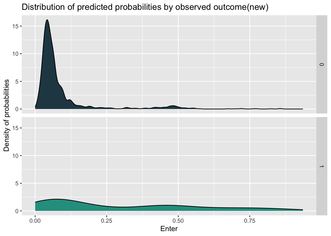

Code

ggplot(testProbs_raw, aes(x = Probs, fill = as.factor(Outcome))) + 
  geom_density() +
  facet_grid(Outcome ~ .) +
  scale_fill_manual(values = palette2) +
  labs(x = "Enter", y = "Density of probabilities",
       title = "Distribution of predicted probabilities by observed outcome(raw)") +
  theme(strip.text.x = element_text(size = 18),
        legend.position = "none")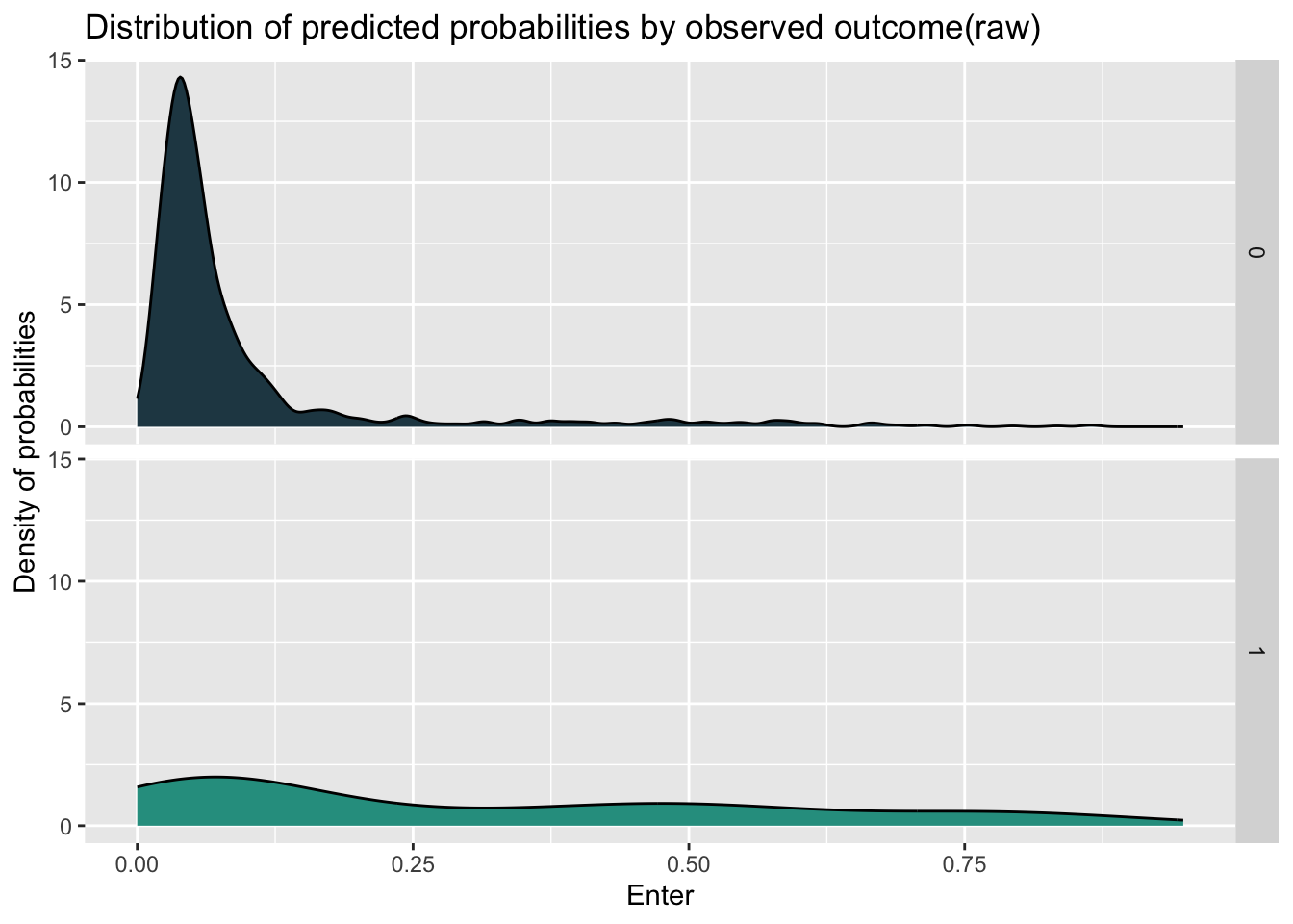

Threshold setting and analysis

Based on the density, I set the probability’s threshold of 0.14 for determine whether the objective will enter the program. From the aspect of sensitivity, which represent the ability to correctly identify positive instances, the new model has better performance than the model with raw feature.

Code

testProbs <- 
  testProbs %>%
  mutate(predOutcome  = as.factor(ifelse(testProbs$Probs > 0.5 , 1, 0)))

caret::confusionMatrix(testProbs$predOutcome, testProbs$Outcome, 
                       positive = "1")

Confusion Matrix and Statistics

          Reference
Prediction    0    1
         0 1256  123
         1   27   34
                                              
               Accuracy : 0.8958              
                 95% CI : (0.8789, 0.9111)    
    No Information Rate : 0.891               
    P-Value [Acc > NIR] : 0.294               
                                              
                  Kappa : 0.2672              
                                              
 Mcnemar's Test P-Value : 0.000000000000008716
                                              
            Sensitivity : 0.21656             
            Specificity : 0.97896             
         Pos Pred Value : 0.55738             
         Neg Pred Value : 0.91080             
             Prevalence : 0.10903             
         Detection Rate : 0.02361             
   Detection Prevalence : 0.04236             
      Balanced Accuracy : 0.59776             
                                              
       'Positive' Class : 1                   
                                              

Code

testProbs_raw <- 
  testProbs_raw %>%
  mutate(predOutcome  = as.factor(ifelse(testProbs_raw$Probs > 0.5 , 1, 0)))

caret::confusionMatrix(testProbs_raw$predOutcome, testProbs_raw$Outcome, 
                       positive = "1")

Confusion Matrix and Statistics

          Reference
Prediction    0    1
         0 1239  113
         1   44   44
                                          
               Accuracy : 0.891           
                 95% CI : (0.8737, 0.9066)
    No Information Rate : 0.891           
    P-Value [Acc > NIR] : 0.5212          
                                          
                  Kappa : 0.3047          
                                          
 Mcnemar's Test P-Value : 0.00000005731   
                                          
            Sensitivity : 0.28025         
            Specificity : 0.96571         
         Pos Pred Value : 0.50000         
         Neg Pred Value : 0.91642         
             Prevalence : 0.10903         
         Detection Rate : 0.03056         
   Detection Prevalence : 0.06111         
      Balanced Accuracy : 0.62298         
                                          
       'Positive' Class : 1               
                                          

ROC Curve & AUC score

To see the performance of two models more directly, I check the ROC(Receiver Operating Characteristic) curve, which visualize the performance of binary classification model. The curve that is “above” the y=x line shows the good performance of model. What’s more, I use the AUC (area under curve) score to measure the behavior, with higher score represent better ability to distinguish between the features. And the model with new feature having higher AUC score indicates the better interpretability for whether entering the program.

Code

ggplot(testProbs, aes(d = as.numeric(Outcome), m = Probs)) +
  geom_roc(n.cuts = 50, labels = FALSE, colour = "#FE9900") +
  style_roc(theme = theme_grey) +
  geom_abline(slope = 1, intercept = 0, size = 1.5, color = 'grey') +
  labs(title = "ROC Curve - clickModel")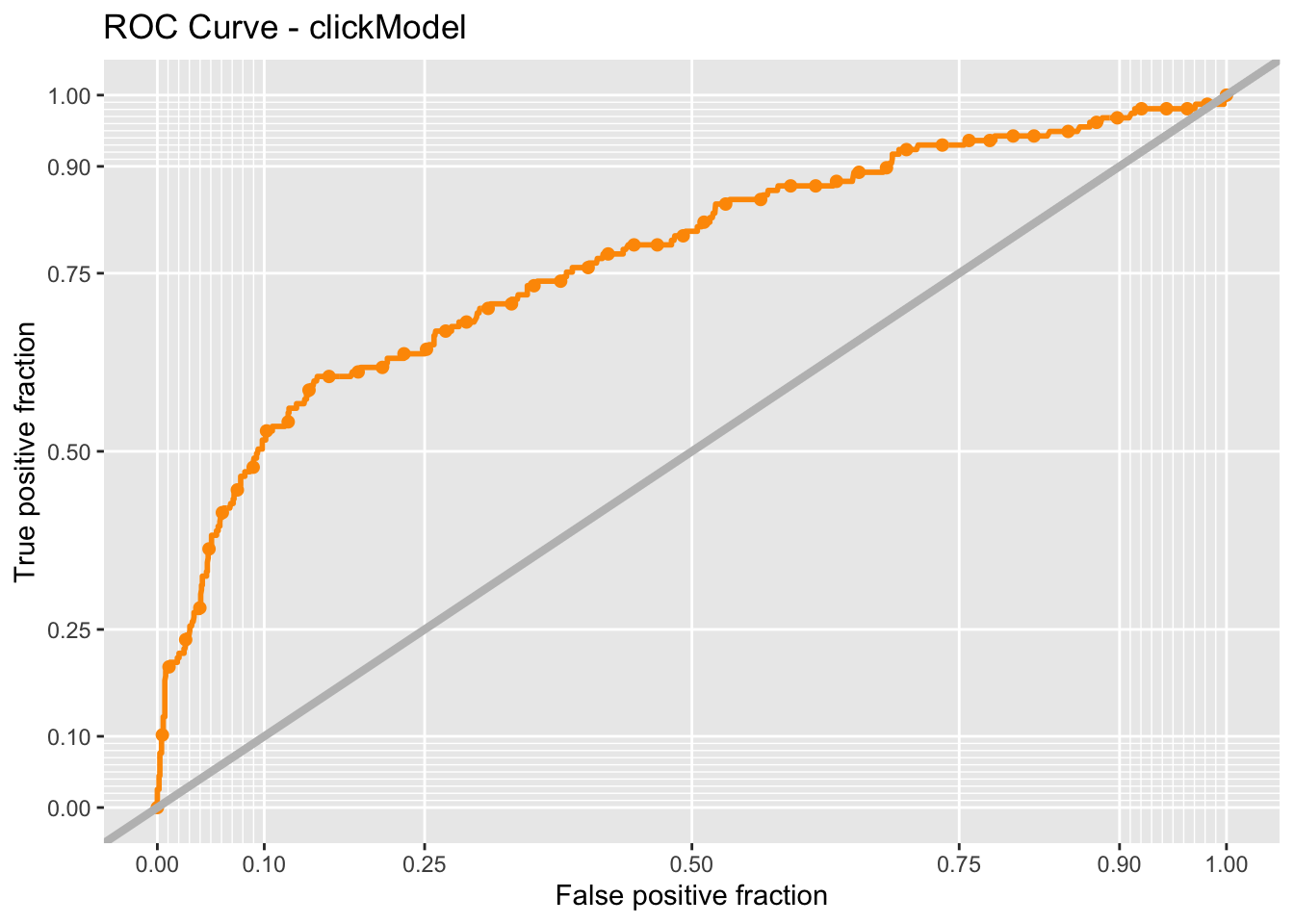

Code

auc(testProbs$Outcome, testProbs$Probs)

Area under the curve: 0.7687

Code

auc(testProbs_raw$Outcome, testProbs_raw$Probs)

Area under the curve: 0.7517

Cross Validation & Fitness

To assess the performance and generalization ability of two models and identify the issue of over-fitting due to randomness of train and test data splitting, I use cross validation to compare and select the final model. Comparing the results of two models, we can find that the the new model in general has better performance due to higher ROC score and sensitivity.

Code

ctrl <- trainControl(method = "cv", number = 100, classProbs=TRUE, summaryFunction=twoClassSummary)

cvFit <- train(y ~ .,
                  data=house_sub %>% 
                    dplyr::select(-X,-y_numeric,-poutcome,-education,-job,-pdays,
                                  -age,-day_of_week,-mortgage,
                                -taxbill_in_phl,-taxLien,-cons.price.idx,-cons.conf.idx), 
                method="glm", family="binomial",
                metric="ROC", trControl = ctrl)

cvFit

Generalized Linear Model 

4119 samples
  14 predictor
   2 classes: 'no', 'yes' 

No pre-processing
Resampling: Cross-Validated (100 fold) 
Summary of sample sizes: 4078, 4078, 4077, 4077, 4079, 4079, ... 
Resampling results:

  ROC        Sens       Spec 
  0.7729003  0.9825676  0.209

Code

cvFit_raw <- train(y ~ .,
                  data=house_sub %>% 
                    dplyr::select(-X,- y_numeric,-cons.price.idx_s,-cons.conf.idx_s,
                                  -poutcome_new,-education_new,-job_new,-pdays_new), 
                method="glm", family="binomial",
                metric="ROC", trControl = ctrl)

cvFit_raw

Generalized Linear Model 

4119 samples
  19 predictor
   2 classes: 'no', 'yes' 

No pre-processing
Resampling: Cross-Validated (100 fold) 
Summary of sample sizes: 4078, 4078, 4077, 4078, 4077, 4078, ... 
Resampling results:

  ROC       Sens       Spec  
  0.762658  0.9811562  0.2185

To check the goodness of fitting metrics more clearly, I visualize the result of 100 times cross validation to see the generalization and stability of the model when confronting different data. From the histogram of ROC score, we can find that the new model has distribution more like normal distribution compared the the raw model, and the situation shows that the new model is relatively more stable across different subsets of the data. What’s more, when we focus on the distribution of sensitivity, the new model has more density on the higher sensitivity score, which shows that the new model has better ability to correctly identify positive instances.

Code

dplyr::select(cvFit$resample, -Resample) %>%
  gather(metric, value) %>%
  left_join(gather(cvFit$results[2:4], metric, mean)) %>%
  ggplot(aes(value)) + 
    geom_histogram(bins=35, fill = "#2a9d8f") +
    facet_wrap(~metric) +
    geom_vline(aes(xintercept = mean), colour = "#e76f51", linetype = 3, size = 1.5) +
    scale_x_continuous(limits = c(0, 1)) +
    labs(x="Goodness of Fit", y="Count", title="CV Goodness of Fit Metrics(new)",
         subtitle = "Across-fold mean reprented as dotted lines")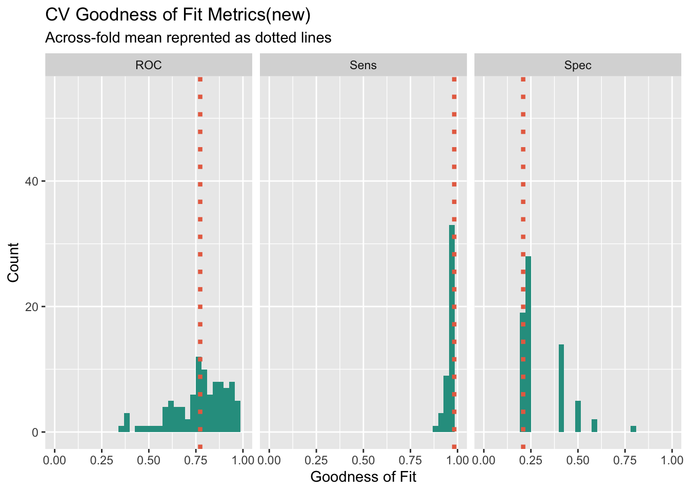

Code

dplyr::select(cvFit_raw$resample, -Resample) %>%
  gather(metric, value) %>%
  left_join(gather(cvFit$results[2:4], metric, mean)) %>%
  ggplot(aes(value)) + 
    geom_histogram(bins=35, fill = "#2a9d8f") +
    facet_wrap(~metric) +
    geom_vline(aes(xintercept = mean), colour = "#e76f51", linetype = 3, size = 1.5) +
    scale_x_continuous(limits = c(0, 1)) +
    labs(x="Goodness of Fit", y="Count", title="CV Goodness of Fit Metrics(old)",
         subtitle = "Across-fold mean reprented as dotted lines")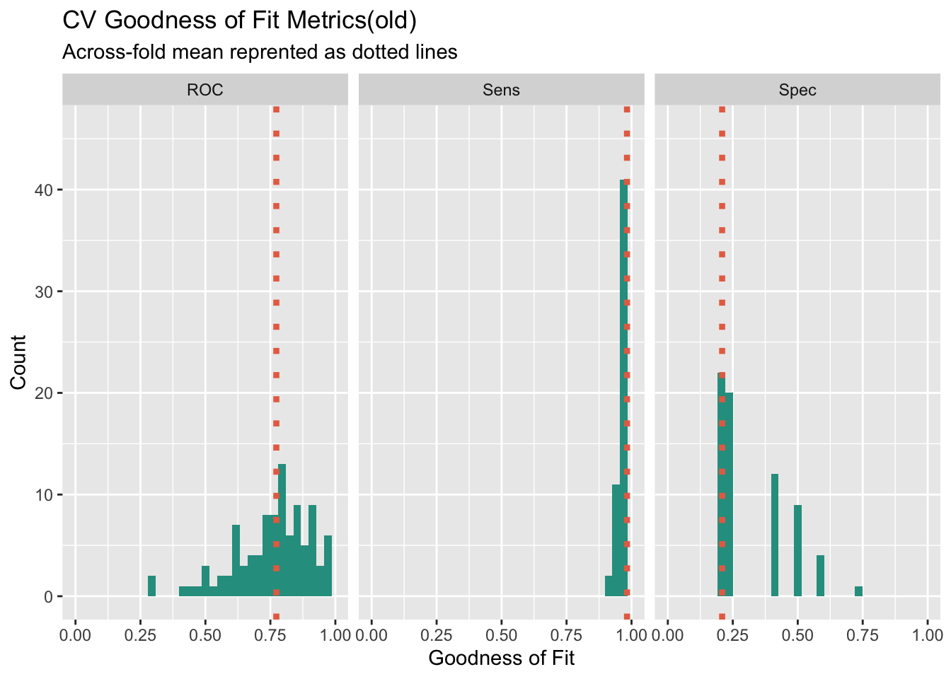

Cost-Benefit Calculation

Situation Definition

To use the model to help calculate the benefits under the prediction of model, we need to set the benefits of different combinations of predicted and actual situation first. Our approach will be to use the confusion matrix from testProbs. Below the cost/benefit for each outcome in our confusion matrix is calculated, like so:

True Negative: $0 True Positive: (-$2850 - $5000 + $10000 + $56000)*0.25*Count - $2850*0.75Count False Negative: -$2850Count False Positive: $0

Cost-Benefit Analysis

From the result of cost/benefit table, we can find that the main benefit comes from True-positive situation, which represent we correctly predict that the homeowner will enter the program. And the main cost comes from False-positive, where we would put into money for marketing source and the homeowners will not enter.

Code

cost_benefit_table <-
   testProbs %>%
      count(predOutcome, Outcome) %>%
      summarize(True_Negative = sum(n[predOutcome==0 & Outcome==0]),
                True_Positive = sum(n[predOutcome==1 & Outcome==1]),
                False_Negative = sum(n[predOutcome==0 & Outcome==1]),
                False_Positive = sum(n[predOutcome==1 & Outcome==0])) %>%
       gather(Variable, Count) %>%
       mutate(Revenue =
               ifelse(Variable == "True_Negative",0,
               ifelse(Variable == "True_Positive",((-2850-5000+10000+56000)*(Count*0.25)+(-2850*Count*0.75)),
               ifelse(Variable == "False_Negative", 0,
               ifelse(Variable == "False_Positive", -2850 * Count, 0))))) %>%
    bind_cols(data.frame(Description = c(
              "We correctly predicted no enter",
              "We correctly predicted enter",
              "We predicted no enter and homeowner want to enter",
              "We predicted homeowner will enter and homeowner did not enter")))

kable(cost_benefit_table,
       caption = "Cost/Benefit Table") %>% kable_styling()

Cost/Benefit Table

Variable	Count	Revenue	Description
True_Negative	1256	0	We correctly predicted no enter
True_Positive	34	421600	We correctly predicted enter
False_Negative	123	0	We predicted no enter and homeowner want to enter
False_Positive	27	-76950	We predicted homeowner will enter and homeowner did not enter

Code

iterateThresholds <- function(data) {
  x = .01
  all_prediction <- data.frame()
  while (x <= 1) {
  
  this_prediction <-
      testProbs %>%
      mutate(predOutcome = ifelse(Probs > x, 1, 0)) %>%
      count(predOutcome, Outcome) %>%
      summarize(True_Negative = sum(n[predOutcome==0 & Outcome==0]),
                True_Positive = sum(n[predOutcome==1 & Outcome==1]),
                False_Negative = sum(n[predOutcome==0 & Outcome==1]),
                False_Positive = sum(n[predOutcome==1 & Outcome==0])) %>%
     gather(Variable, Count) %>%
     mutate(Revenue =
               ifelse(Variable == "True_Negative", 0,
               ifelse(Variable == "True_Positive",((-2850-5000+10000+56000)*(Count*0.25)+(-2850*Count*0.75)),
               ifelse(Variable == "False_Negative", 0,
               ifelse(Variable == "False_Positive", -2850 * Count, 0)))),
            Threshold = x)
  
  all_prediction <- rbind(all_prediction, this_prediction)
  x <- x + .01
  }
return(all_prediction)
}

Based on the cost/benefit analysis, we want to increase the true-positive rate and decrease the False-Positive rate to increase the total benefit for the model.Therefore, we need to find the different threshold’s influence on this two indicators. We can find that with the increase of threshold, the True-positive and False Positive will both decrease.

Code

whichThreshold <- iterateThresholds(test_Probs1)

whichThreshold %>%
  ggplot(.,aes(Threshold, Count, colour = Variable)) +
  geom_point() +
  scale_colour_manual(values = palette4) +    
  labs(title = "Confusion Metric Outcome by Threshold",
       y = "Count") +
  guides(colour=guide_legend(title = "Legend"))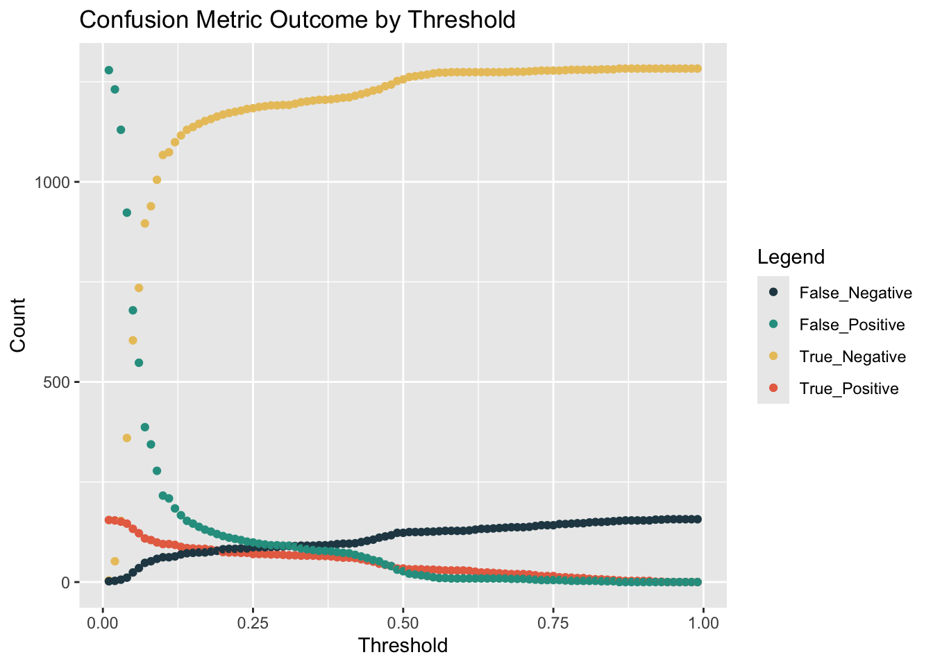 

However, it’s hard to get the maximium of benefits easily. So we plot the line of benefits with the increasing threshold. We can find the benefit will reach the max when the threshold is set as 0.14 properly.

Code

whichThreshold <- iterateThresholds(testProbs2)

whichThreshold_revenue <- 
whichThreshold %>% 
    group_by(Threshold) %>% 
    summarize(Revenue = sum(Revenue))

  ggplot(whichThreshold_revenue)+
  geom_line(aes(x = Threshold, y = Revenue))+
  geom_vline(xintercept =  pull(arrange(whichThreshold_revenue, -Revenue)[1,1]))+
    labs(title = "Model Revenues By Threshold For Test Sample",
         subtitle = "Vertical Line Denotes Optimal Threshold")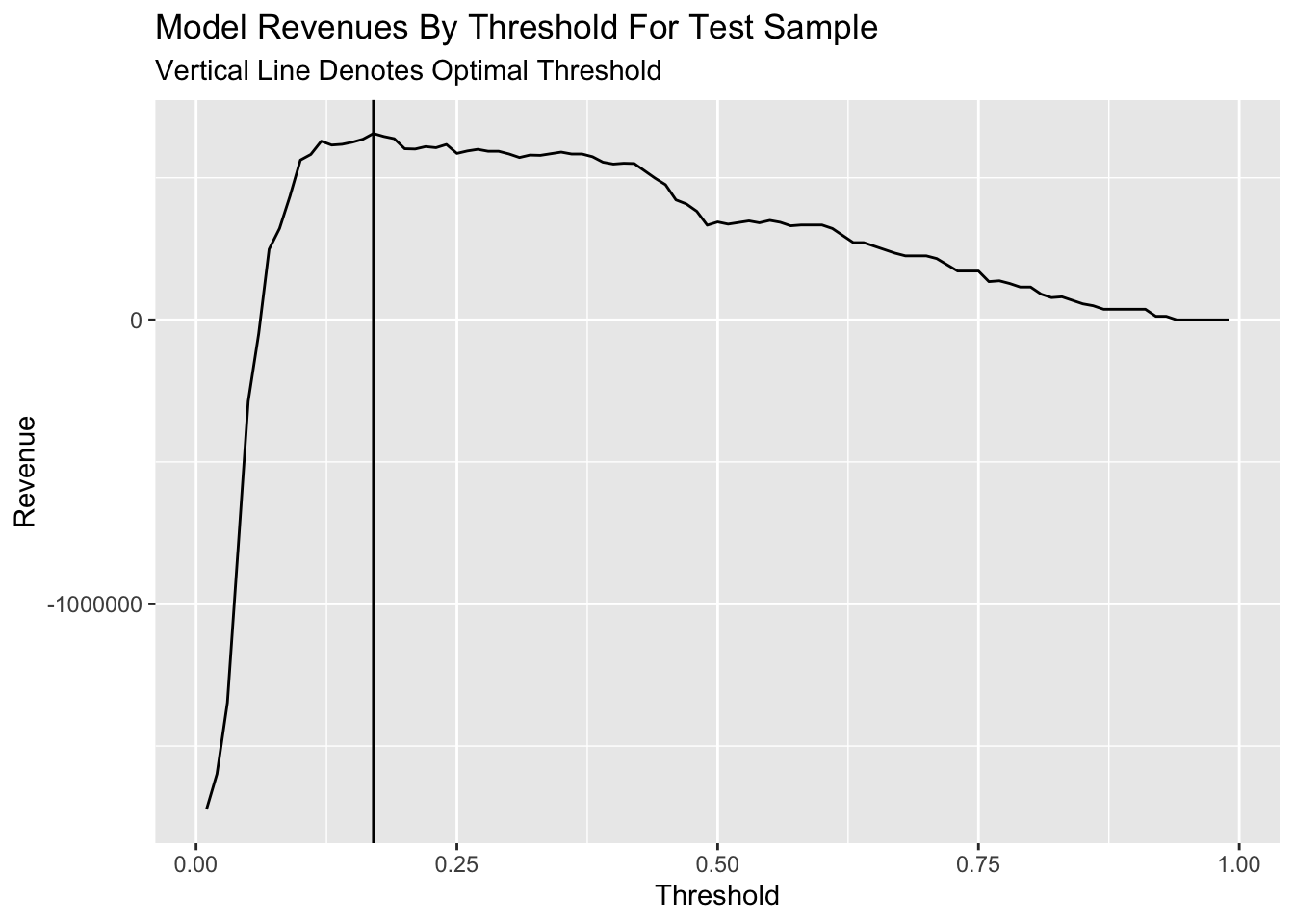

However, if we use the counts of credits, which represents the number of homeowners can get the credit to enter the program, to measure the performance of different threshold, we can find that the count of credit will continously increase with the increase of threshold until the threshold comes to 0.8.

Code

whichThreshold_credit <- 
whichThreshold %>% 
  mutate(credit =  ifelse(Variable == "True_Positive", (Count * 0.25),
                             ifelse(Variable == "False_Negative", Count, 0))) %>%
  group_by(Threshold) %>% 
  summarize(Credit = sum(credit))

  ggplot(whichThreshold_credit)+
  geom_line(aes(x = Threshold, y = Credit, colour = "#FE9900"))+
  geom_vline(xintercept =  pull(arrange(whichThreshold_credit, -Credit)[1,1]))+
    labs(title = "Total Count of Credits By Threshold For Test Sample",
         subtitle = "Vertical Line Denotes Optimal Threshold")+
  theme(legend.position = "None")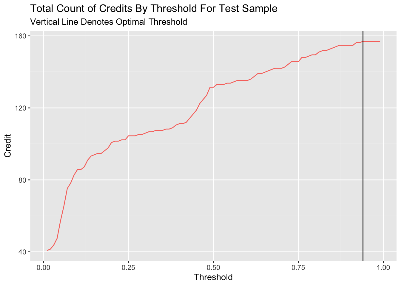

if we compare the revenue and credit number of the optimal benefits’ threshold and 0.5 threshold, we can find that despite the benefit will reach max with 0.22 threshold for the model, the model with serve less credit compared to 0.5 threshold.

Code

threshold_table <- merge(whichThreshold_revenue, whichThreshold_credit, by = "Threshold")

final_table <- threshold_table %>%
                  slice(22, 50) 

kable(final_table, caption = "Total Revenue and Total Count of Credits for Optimal Threshold and 0.5 Threshold") %>% 
  kable_styling()

Total Revenue and Total Count of Credits for Optimal Threshold and 0.5 Threshold

Threshold	Revenue	Credit
0.22	609800	101.5
0.50	344650	131.5

Conclusion

In general, I would not recommend this model be put into production. For one thing, the model could have potential bias due to the feature used in the model. The reclassification and consideration of martial, job, and education would lead to potential bias to the vulnerable group in the model production. What’s more, the model show the weakness in the reliability due to model’s low likelihood. This situation may come from limited features in the dataset. If the model could consider more comprehensive factors that influence the credit of homeowner, the model could have better likelihood performance.

Therefore, to improve the performance of model, we can add more variables in the model to increase the comprehensive consideration. For another, we could also think about the features which could lead to bias more consciously. To ensure that the marketing materials resulted in a better response rate, we could based on the actual situation to switch the threshold of model promptly based on the period feedback from the market.